Ch2 预备知识

望秋弥茂2023-12-072023-12-15

2.1数据操作

2.1.5 节省内存

⽤X[:] = X + Y或X += Y来减少操作的内存开销
1
2
X[:] = X + Y
X += Y

2.2 数据预处理

2.2.1 读取数据集

# 写入数据
import os
os.makedirs(os.path.join('..', 'data'), exist_ok=True)
data_file = os.path.join('..', 'data', 'house_tiny.csv') # ../data/house_tiny.csv
with open(data_file, 'w') as f:
	f.write('NumRooms,Alley,Price\n') # 列名
	f.write('NA,Pave,127500\n') # 每⾏表⽰⼀个数据样本
	f.write('2,NA,106000\n')

# 读取数据集
import pandas as pd
data = pd.read_csv(data_file)

2.2.2 处理缺失值

1
2

inputs = inputs.fillna(inputs.mean()) # 同⼀列的均值替换“NaN”项
inputs = pd.get_dummies(inputs, dummy_na=True) # 自动将input的将此列转换为非NaN的值以及NaN，取值为0，1

2.2.3 转换为张量格式

1
2
3

import torch

X, y = torch.tensor(inputs.values), torch.tensor(outputs.values) # input,output都是数值条目

2.3 线性代数

2.3.2 向量

1
2
3

x[3] # 访问索引元素
len(x) # 长度
x.shape # 维度

张量的维度用来表示张量具有的轴数

2.3.3 矩阵

1 2	A = torch.arange(20, dtype=torch.float32).reshape(5, 4) # 更改维度5×4 A.T # 转置

2.3.4 张量

1	X = torch.arange(24).reshape(2, 3, 4) # 2个3×4的矩阵

2.3.5 张量算法的基本性质

2.3.6 降维

A = (tensor([[ 0., 1., 2., 3.],
			 [ 4., 5., 6., 7.],
			 [ 8., 9., 10., 11.],
			 [12., 13., 14., 15.],
			 [16., 17., 18., 19.]]),

1 2	A_sum_axis0 = A.sum(axis=0) A_sum_axis0, A_sum_axis0.shape

1	(tensor([40., 45., 50., 55.]), torch.Size([4]))

1 2	A_sum_axis1 = A.sum(axis=1) A_sum_axis1, A_sum_axis1.shape

1	(tensor([ 6., 22., 38., 54., 70.]), torch.Size([5]))

1 2	A.sum(axis=[0, 1]) # 结果和A.sum()相同 A.mean(axis=[0, 1]) # mean也有一样的语法

非降维求和

1	sum_A = A.sum(axis=1, keepdims=True)

tensor([[ 6.],
		[22.],
		[38.],
		[54.],
		[70.]])

sum_A在对每⾏进⾏求和后仍保持两个轴, 直接除可以获得每一行自己的平均数，元素/该行总和
1
A / sum_A

某个轴进行累积求和

1	A.cumsum(axis=0)

tensor([[ 0., 1., 2., 3.],
		[ 4., 6., 8., 10.],
		[12., 15., 18., 21.],
		[24., 28., 32., 36.],
		[40., 45., 50., 55.]])

2.3.7 点积

1 2	torch.dot(x, y) torch.sum(x * y)

2.3.8 矩阵-向量积

1	A.shape, x.shape, torch.mv(A, x)

1	(torch.Size([5, 4]), torch.Size([4]), tensor([ 14., 38., 62., 86., 110.]))

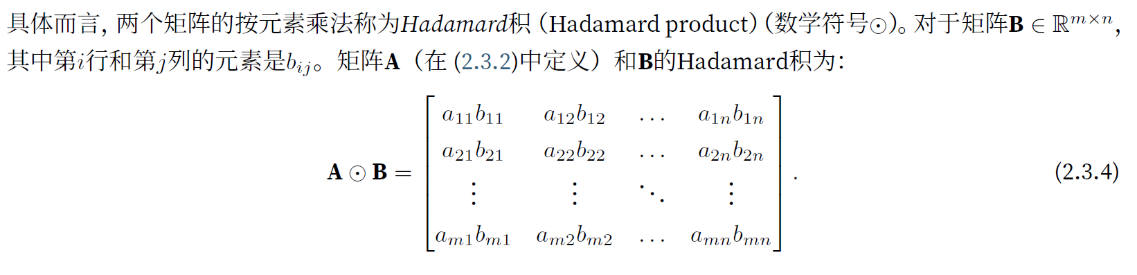
2.3.9 矩阵-矩阵乘法

1	torch.mm(A, B) # 标准矩阵乘法，与Hadamard积（点对点乘积）不同

2.3.10 范数

$L_2$ 范数中常常省略下标2，也就是说 $||x||$ 等同于 $||x||_2$
$$
|\mathbf{x}|2=\sqrt{\sum{i=1}^n x_i^2}
$$

1	torch.norm(u)

$L_1$ 范数
$$
|\mathbf{x}|1=\sum{i=1}^n\left|x_i\right|
$$

1	torch.abs(u).sum()

$L_p$ 范数定义
$$
|\mathbf{x}|p=\left(\sum{i=1}^n\left|x_i\right|^p\right)^{1 / p}
$$
Frobenius 范数
- Frobenius范数满⾜向量范数的所有性质，它就像是矩阵形向量的 $L_2$ 范数。
  $$
  |\mathbf{X}|F=\sqrt{\sum{i=1}^m \sum_{j=1}^n x_{i j}^2}
  $$

1	torch.norm(torch.ones((4, 9)))

练习

1.证明⼀个矩阵 $A$ 的转置的转置是A，即 $(A^T)^T = A$

对于每一个元素定义易证

2.给出两个矩阵 $A$ 和 $B$ ，证明“它们转置的和”等于“它们和的转置”，即$A^T+B^T=(A+B)^T$

对于每一个元素定义易证

3.给定任意⽅阵 $A$ ， $A+A^T$ 总是对称的吗?为什么?

对于每一个元素定义易证

4.本节中定义了形状(2; 3; 4)的张量X。len(X)的输出结果是什么？

1
2
3

X = torch.ones(2, 3, 4)

print(len(X))

5.对于任意形状的张量X, len(X)是否总是对应于X特定轴的⻓度?这个轴是什么?

对应shape的第一个轴的数目，axis=0

6.运⾏A/A.sum(axis=1)，看看会发⽣什么。请分析⼀下原因？

矩阵除以一维张量，要看矩阵列数是否等于张量的元素个数（也可以看作是列数）是否相等，如果相等就可以实现，将矩阵该列的所有元素除以对应列的张量元素。否则会报错

A = torch.arange(20).reshape(5, 4)

print(A, A.shape)
print(A.sum(axis=0), A.sum(axis=0).shape)
print(A/A.sum(axis=0), (A/A.sum(axis=0)).shape)
print(A.sum(axis=1), A.sum(axis=1).shape)
print(A.sum(axis=1, keepdims=True), A.sum(axis=1, keepdims=True).shape)
print(A/A.sum(axis=1, keepdims=True), (A/A.sum(axis=1, keepdims=True)).shape)
print(A/A.sum(axis=1), (A/A.sum(axis=1)).shape)

tensor([[ 0, 1, 2, 3], 
		[ 4, 5, 6, 7], 
		[ 8, 9, 10, 11], 
		[12, 13, 14, 15], 
		[16, 17, 18, 19]]) torch.Size([5, 4]) 
tensor([40, 45, 50, 55]) torch.Size([4]) 
tensor([[0.0000, 0.0222, 0.0400, 0.0545], 
		[0.1000, 0.1111, 0.1200, 0.1273], 
		[0.2000, 0.2000, 0.2000, 0.2000], 
		[0.3000, 0.2889, 0.2800, 0.2727], 
		[0.4000, 0.3778, 0.3600, 0.3455]]) torch.Size([5, 4]) 
tensor([ 6, 22, 38, 54, 70]) torch.Size([5]) 
tensor([[ 6], [22], [38], [54], [70]]) torch.Size([5, 1]) 
tensor([[0.0000, 0.1667, 0.3333, 0.5000], 
		[0.1818, 0.2273, 0.2727, 0.3182], 
		[0.2105, 0.2368, 0.2632, 0.2895], 
		[0.2222, 0.2407, 0.2593, 0.2778], 
		[0.2286, 0.2429, 0.2571, 0.2714]]) torch.Size([5, 4])

7.考虑⼀个具有形状(2; 3; 4)的张量，在轴0、1、2上的求和输出是什么形状?

三维张量可以视作一个空间矩阵，然后分别沿着axis（第一个0，依次递增）进行降维求和，减少的是对应axis方向的维度。

X = torch.arange(24).reshape(2, 3, 4)

print(X, X.shape)
print(X.sum(axis=0), X.sum(axis=0).shape)
print(X.sum(axis=1), X.sum(axis=1).shape)
print(X.sum(axis=2), X.sum(axis=2).shape)

tensor([[[ 0, 1, 2, 3], 
		 [ 4, 5, 6, 7], 
		 [ 8, 9, 10, 11]], 
		 
		[[12, 13, 14, 15], 
		 [16, 17, 18, 19], 
		 [20, 21, 22, 23]]]) torch.Size([2, 3, 4]) 
tensor([[12, 14, 16, 18], 
		[20, 22, 24, 26], 
		[28, 30, 32, 34]]) torch.Size([3, 4]) 
tensor([[12, 15, 18, 21], 
		[48, 51, 54, 57]]) torch.Size([2, 4]) 
tensor([[ 6, 22, 38], 
		[54, 70, 86]]) torch.Size([2, 3])

8.为linalg.norm函数提供3个或更多轴的张量，并观察其输出。对于任意形状的张量这个函数计算得到什么?

本质就是在求每个元素的平方和的平方根结果。

X = torch.ones(2, 3, 4)
X = X.numpy()
print(X)
print(np.linalg.norm(X))

[[[1. 1. 1. 1.] 
  [1. 1. 1. 1.] 
  [1. 1. 1. 1.]] 
  
 [[1. 1. 1. 1.] 
  [1. 1. 1. 1.] 
  [1. 1. 1. 1.]]] 
4.8989797 
4.898979485566356

2.4 微积分

将拟合模型的任务分解为两个关键问题：
1. #优化（optimization）：⽤模型拟合观测数据的过程
2. #泛化（generalization）：数学原理和实践者的智慧，能够指导我们⽣成出有效性超出⽤于训练的数据集本⾝的模型。

2.4.1 导数与微分

#@save是⼀个特殊的标记，会将对应的函数、类或语句保存在d2l包中

set_axes函数⽤于设置由matplotlib⽣成图表的轴的属性。

#@save
def set_axes(axes, xlabel, ylabel, xlim, ylim, xscale, yscale, legend):
	"""设置matplotlib的轴"""
	axes.set_xlabel(xlabel)
	axes.set_ylabel(ylabel)
	axes.set_xscale(xscale)
	axes.set_yscale(yscale)
	axes.set_xlim(xlim)
	axes.set_ylim(ylim)
	if legend:
		axes.legend(legend)
	axes.grid()

定义⼀个plot函数来简洁地绘制多条曲线

#@save
def plot(X, Y=None, xlabel=None, ylabel=None, legend=None, xlim=None,
		 ylim=None, xscale='linear', yscale='linear',
		 fmts=('-', 'm--', 'g-.', 'r:'), figsize=(3.5, 2.5), axes=None):
	"""绘制数据点"""
	if legend is None:
		legend = []
		
	set_figsize(figsize)
	axes = axes if axes else d2l.plt.gca()
	
	# 如果X有⼀个轴，输出True
	def has_one_axis(X):
		return (hasattr(X, "ndim") and X.ndim == 1 or isinstance(X, list)
				and not hasattr(X[0], "__len__"))
				
	if has_one_axis(X):
		X = [X]
	if Y is None:
		X, Y = [[]] * len(X), X
	elif has_one_axis(Y):
		Y = [Y]
	if len(X) != len(Y):
		X = X * len(Y)
	axes.cla()
	for x, y, fmt in zip(X, Y, fmts):
		if len(x):
			axes.plot(x, y, fmt)
		else:
			axes.plot(y, fmt)
	set_axes(axes, xlabel, ylabel, xlim, ylim, xscale, yscale, legend)

2.4.2 偏导数

$$ \frac{\partial y}{\partial x_i} = \lim_{h \rightarrow 0} \frac{f(x_1, \ldots, x_{i-1}, x_i+h, x_{i+1}, \ldots, x_n) - f(x_1, \ldots, x_i, \ldots, x_n)}{h}.$$

对于偏导数的表示，以下是等价的：
$$\frac{\partial y}{\partial x_i} = \frac{\partial f}{\partial x_i} = f_{x_i} = f_i = D_i f = D_{x_i} f.$$

2.4.3 梯度

设函数$f:\mathbb{R}^n\rightarrow\mathbb{R}$的输入是一个$n$维向量$\mathbf{x}=[x_1,x_2,\ldots,x_n]^\top$，并且输出是一个标量。
函数$f(\mathbf{x})$相对于$\mathbf{x}$的梯度是一个包含$n$个偏导数的向量:
$$\nabla_{\mathbf{x}} f(\mathbf{x}) = \bigg[\frac{\partial f(\mathbf{x})}{\partial x_1}, \frac{\partial f(\mathbf{x})}{\partial x_2}, \ldots, \frac{\partial f(\mathbf{x})}{\partial x_n}\bigg]^\top$$
其中$\nabla_{\mathbf{x}} f(\mathbf{x})$通常在没有歧义时被$\nabla f(\mathbf{x})$取代。
假设$\mathbf{x}$为$n$维向量，在微分多元函数时经常使用以下规则:
1. 对于所有$\mathbf{A} \in \mathbb{R}^{m \times n}$，都有$\nabla_{\mathbf{x}} \mathbf{A} \mathbf{x} = \mathbf{A}^\top$
2. 对于所有$\mathbf{A} \in \mathbb{R}^{n \times m}$，都有$\nabla_{\mathbf{x}} \mathbf{x}^\top \mathbf{A} = \mathbf{A}$
3. 对于所有$\mathbf{A} \in \mathbb{R}^{n \times n}$，都有$\nabla_{\mathbf{x}} \mathbf{x}^\top \mathbf{A} \mathbf{x} = (\mathbf{A} + \mathbf{A}^\top)\mathbf{x}$
4. $\nabla_{\mathbf{x}} |\mathbf{x} |^2 = \nabla_{\mathbf{x}} \mathbf{x}^\top \mathbf{x} = 2\mathbf{x}$
同样，对于任何矩阵$\mathbf{X}$，都有$\nabla_{\mathbf{X}} |\mathbf{X} |_F^2 = 2\mathbf{X}$。

2.4.4 链式法则

练习

1.绘制函数$y = f(x) = x^3 - \frac{1}{x}$和其在$x = 1$处切线的图像。

def f(x):
    return x ** 3 - 1/x
    
x = np.arange(0.1, 3, 0.1)

plot(x, [f(x), 4*x-4], 'x', 'f(x)', legend=['f(x)', 'Tangent line (x=1)'])

2.求函数$f(\mathbf{x}) = 3x_1^2 + 5e^{x_2}$的梯度。

$$
\nabla_{\mathbf{x}} f(\mathbf{x}) = [6x_1, 5e^{x_2}]^\top
$$

3.函数$f(\mathbf{x}) = |\mathbf{x}|_2$的梯度是什么？

二范数定义如下

$$
|\mathbf{x}|2=\sqrt{\sum{i=1}^n x_i^2}
$$

证明如下

$$
\begin{equation}
\begin{aligned}
\nabla f(\mathbf{x}) &= \nabla |\mathbf{x}|2 \
& =\nabla \sqrt{\sum{i=1}^n x_i^2} \
& =\bigg[\frac{\partial f(\mathbf{x})}{\partial x_1}, \frac{\partial f(\mathbf{x})}{\partial x_2}, \ldots, \frac{\partial f(\mathbf{x})}{\partial x_n}\bigg]^\top \
& =\bigg[\frac{\partial \sqrt{\sum_{i=1}^n x_i^2} }{\partial x_1}, \frac{\partial \sqrt{\sum_{i=1}^n x_i^2} }{\partial x_2}, \ldots, \frac{\partial \sqrt{\sum_{i=1}^n x_i^2} }{\partial x_n}\bigg]^\top \
& = \frac{1}{2|\mathbf{x}|_2}\bigg[2(x_1), 2(x_2), \ldots, 2(x_n)\bigg]^\top \
& = \frac{1}{|\mathbf{x}|_2}\bigg[x_1, x_2, \ldots, x_n\bigg]^\top \
& = \frac{\mathbf{x}}{|\mathbf{x}|_2}
\end{aligned}
\end{equation}
$$

4.尝试写出函数$u = f(x, y, z)$，其中$x = x(a, b)$，$y = y(a, b)$，$z = z(a, b)$的链式法则。

$$
\begin{align}
\frac{\partial u}{\partial a} = \frac{\partial u}{\partial x}\frac{\partial x}{\partial a}+\frac{\partial u}{\partial y}\frac{\partial y}{\partial a}+\frac{\partial u}{\partial z}\frac{\partial z}{\partial a} \
\frac{\partial u}{\partial a} = \frac{\partial u}{\partial x}\frac{\partial x}{\partial a}+\frac{\partial u}{\partial y}\frac{\partial y}{\partial a}+\frac{\partial u}{\partial z}\frac{\partial z}{\partial a}
\end{align}
$$

2.5 自动微分

2.5.0 深度学习框架

通过⾃动计算导数，即⾃动微分（automatic differentiation）来加快求导。
根据设计好的模型，系统会构建⼀个计算图（computational graph），来跟踪计算是哪些数据通过哪些操作组合起来产⽣输出。
⾃动微分使系统能够随后反向传播梯度。这⾥，反向传播（backpropagate） 意味着跟踪整个计算图，填充关于每个参数的偏导数。

2.5.1 ⼀个简单的例⼦

x.requires_grad_(True) # 等价于x=torch.arange(4.0,requires_grad=True)
x.grad # 默认值是None

y.backward() # 调用反向传播函数
x.grad # 对于x分量的梯度

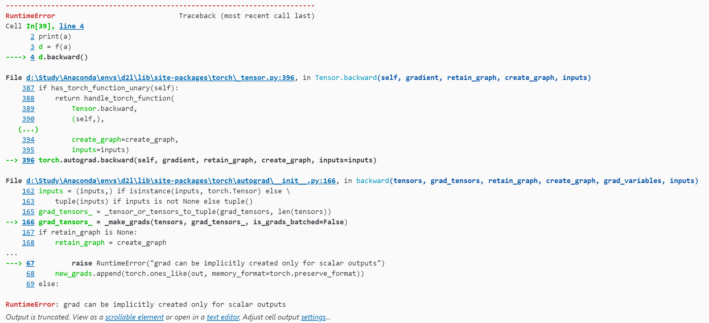
2.5.2 ⾮标量变量的反向传播

在默认情况下，PyTorch会累积梯度，需要清除之前的值
1
2
3
4
x.grad.zero_()
# y = x.sum()
y.backward()
x.grad

2.5.3 分离计算

将某些计算移动到记录的计算图之外
- eg: 假设y是作为x的函数计算的，⽽z则是作为y和x的函数计算的。想象⼀下，我们想计算z关于x的梯度，但由于某种原因，希望将y视为⼀个常数
- 分离y来返回⼀个新变量u，该变量与y具有相同的值，但丢弃计算图中如何计算y的任何信息
- 梯度不会向后流经u到x
  1
  2
  3
  4
  5
  6
  x.grad.zero_()
  y = x * x
  u = y.detach() # 分离计算，设置u变量，但仅使用值，不考虑如何计算的，从而避免x的反向传播
  z = u * x
  z.sum().backward()
  x.grad == u
  1
  tensor([True, True, True, True])

2.5.4 Python控制流的梯度计算

使⽤⾃动微分的⼀个好处是：即使构建函数的计算图需要通过Python控制流（例如，条件、循环或任意函数调⽤），仍然可以计算得到的变量的梯度

练习

为什么计算⼆阶导数⽐⼀阶导数的开销要更⼤？
- 二阶相当于再复用一阶导数的计算
在运⾏反向传播函数之后，⽴即再次运⾏它，看看会发⽣什么。
- 会报错RunTimeError
- 两次backward
在控制流的例⼦中，我们计算d关于a的导数，如果将变量a更改为随机向量或矩阵，会发⽣什么？
- 会报错RunTimeError
- 只支持标量的grad
重新设计⼀个求控制流梯度的例⼦，运⾏并分析结果。
- 暂无
使$f(x)=\sin(x)$，绘制$f(x)$和$\frac{df(x)}{dx}$的图像，其中后者不使用$f’(x)=\cos(x)$。
1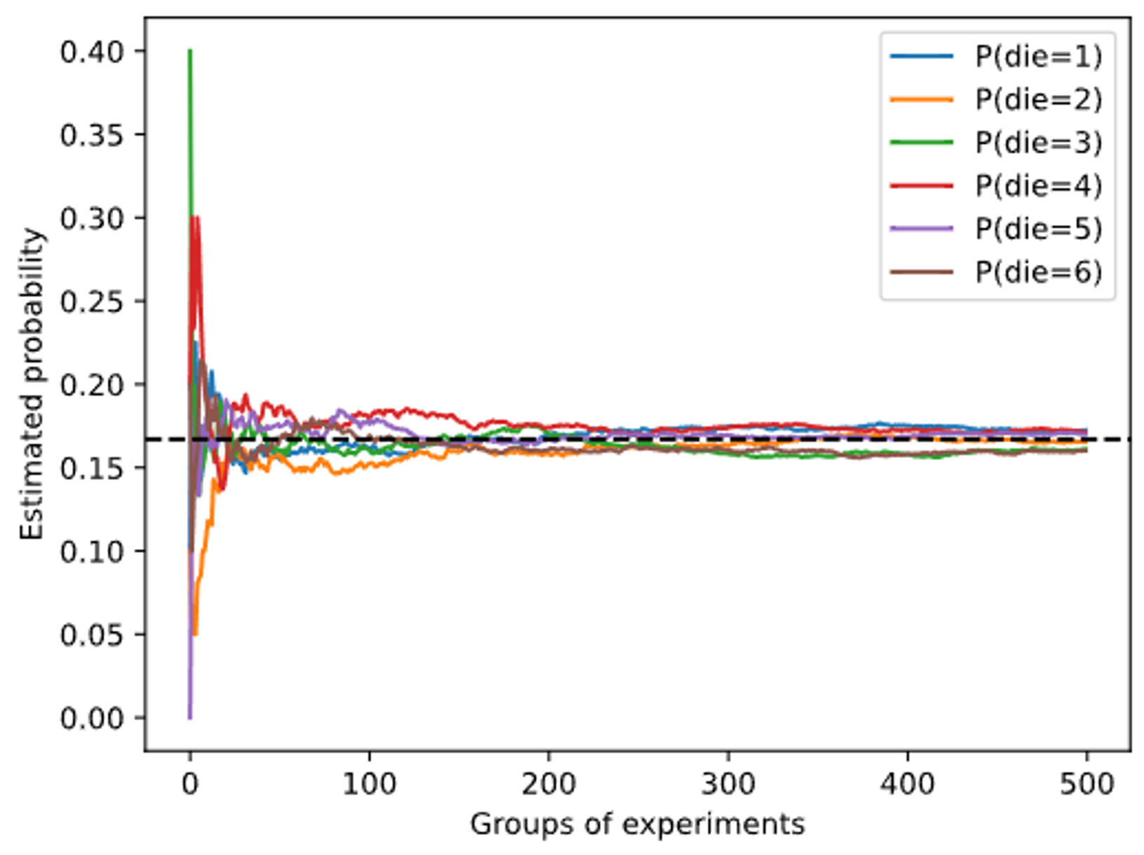

2.6 概率

2.6.1 基本概率论

%matplotlib inline
import torch
from torch.distributions import multinomial
from d2l import torch as d2l

# 投骰子
fair_probs = torch.ones([6]) / 6 # 1-6的概率都是1/6
multinomial.Multinomial(1, fair_probs).sample() # 1次的模拟结果 tensor
multinomial.Multinomial(10, fair_probs).sample() # 10次的模拟结果 tensor

counts = multinomial.Multinomial(10, fair_probs).sample((500,))
cum_counts = counts.cumsum(dim=0)
estimates = cum_counts / cum_counts.sum(dim=1, keepdims=True)
d2l.set_figsize((6, 4.5))
for i in range(6):
	d2l.plt.plot(estimates[:, i].numpy(),
	label=("P(die=" + str(i + 1) + ")"))
d2l.plt.axhline(y=0.167, color='black', linestyle='dashed')
d2l.plt.gca().set_xlabel('Groups of experiments')
d2l.plt.gca().set_ylabel('Estimated probability')
d2l.plt.legend();

概率论公理
1. 概率非负性
2. P(S) = 1 {S: Sample Space}
3. 互斥事件概率为单个事件发生概率之和
随机变量
1. 离散随机变量
2. 连续随机变量

2.6.2 处理多个随机变量

联合概率 (Joint Probability)
条件概率 (Conditional Probability)

$$P(B = b | A = a)$$

乘法法则 (Multiplication Rule)

$$
P(A;B) = P(B|A)P(A)
$$

⻉叶斯定理 (Bayes’ Theorem)

$$
P(A|B) = \frac{P(B|A)P(A)}{P(B)}
$$

边缘化 (Marginalization)

$$
P(B) = \sum_{A}{P(A,B)}
$$

独⽴性 (Independence)

$$
P(A,B) = P(A)P(B)
$$

2.6.3 期望和⽅差

期望 (Expectation)

$$
E[X] = \sum_x{x P(X=x)} \qquad \text{离散随机变量}
$$
$$
E[X] = \int_x{x P(X=x)} \qquad \text{连续随机变量}
$$

方差 (Variance)

$$
Var[X] = E[(X - E(X))^2] = E(X^2) - E(X)^2
$$

练习

进行$m=500$组实验，每组抽取$n=10$个样本。改变$m$和$n$，观察和分析实验结果。
- Center Limit Theorem 中心极限定理
给定两个概率为$P(\mathcal{A})$和$P(\mathcal{B})$的事件，计算$P(\mathcal{A} \cup \mathcal{B})$和$P(\mathcal{A} \cap \mathcal{B})$的上限和下限。（提示：使用友元图来展示这些情况。)
$$
max{({P(\mathcal{A}),P({\mathcal{B}}}))} \leq P(\mathcal{A} \cup \mathcal{B}) \leq P(\mathcal{A} )+P(\mathcal{B} )
$$
$$
0 \leq P(\mathcal{A} \cap \mathcal{B}) \leq min{({P(\mathcal{A}),P({\mathcal{B}}}))} )
$$
假设我们有一系列随机变量，例如$A$、$B$和$C$，其中$B$只依赖于$A$，而$C$只依赖于$B$，能简化联合概率$P(A, B, C)$吗？（提示：这是一个马尔可夫链。)
$$
\begin{equation}
\begin{aligned}
P(A,B,C) &= P(C|B)*P(B) \
&=P(C|B)*P(B|A)*P(A)
\end{aligned}
\end{equation}
$$
在2.6.2节中，第一个测试更准确。为什么不运行第一个测试两次，而是同时运行第一个和第二个测试?
- 也许是成本问题，只需要第二次的不精准测试，也可以大幅度提高推理在阳性反应下，患者真实患病的概率。同时可以避免，同种测试方法可能存在的误差和不为人知的错误。

2.1数据操作

2.1.5 节省内存

2.2 数据预处理

2.2.1 读取数据集

2.2.2 处理缺失值

2.2.3 转换为张量格式

2.3 线性代数

2.3.2 向量

2.3.3 矩阵

2.3.4 张量

2.3.5 张量算法的基本性质

2.3.6 降维

非降维求和

2.3.7 点积

2.3.8 矩阵-向量积

2.3.9 矩阵-矩阵乘法

2.3.10 范数

练习

1.证明⼀个矩阵 $A$ 的转置的转置是A，即 $(A^T)^T = A$

对于每一个元素定义易证

2.给出两个矩阵 $A$ 和 $B$ ，证明“它们转置的和”等于“它们和的转置”，即$A^T+B^T=(A+B)^T$

对于每一个元素定义易证

3.给定任意⽅阵 $A$ ， $A+A^T$ 总是对称的吗?为什么?

对于每一个元素定义易证

4.本节中定义了形状(2; 3; 4)的张量X。len(X)的输出结果是什么？

5.对于任意形状的张量X, len(X)是否总是对应于X特定轴的⻓度?这个轴是什么?

对应shape的第一个轴的数目，axis=0

6.运⾏A/A.sum(axis=1)，看看会发⽣什么。请分析⼀下原因？

7.考虑⼀个具有形状(2; 3; 4)的张量，在轴0、1、2上的求和输出是什么形状?

三维张量可以视作一个空间矩阵，然后分别沿着axis（第一个0，依次递增）进行降维求和，减少的是对应axis方向的维度。

8.为linalg.norm函数提供3个或更多轴的张量，并观察其输出。对于任意形状的张量这个函数计算得到什么?

本质就是在求每个元素的平方和的平方根结果。

2.4 微积分

将拟合模型的任务分解为两个关键问题：

2.4.1 导数与微分

2.4.2 偏导数

2.4.3 梯度

2.4.4 链式法则

练习

1.绘制函数$y = f(x) = x^3 - \frac{1}{x}$和其在$x = 1$处切线的图像。

2.求函数$f(\mathbf{x}) = 3x_1^2 + 5e^{x_2}$的梯度。

3.函数$f(\mathbf{x}) = |\mathbf{x}|_2$的梯度是什么？

二范数定义如下

证明如下

4.尝试写出函数$u = f(x, y, z)$，其中$x = x(a, b)$，$y = y(a, b)$，$z = z(a, b)$的链式法则。

2.5 自动微分

2.5.0 深度学习框架

2.5.1 ⼀个简单的例⼦

2.5.2 ⾮标量变量的反向传播

2.5.3 分离计算

将某些计算移动到记录的计算图之外

2.5.4 Python控制流的梯度计算

练习

会报错RunTimeError

会报错RunTimeError

2.6 概率

2.6.1 基本概率论

概率论公理

随机变量

2.6.2 处理多个随机变量

联合概率 (Joint Probability)

条件概率 (Conditional Probability)

乘法法则 (Multiplication Rule)

⻉叶斯定理 (Bayes’ Theorem)

边缘化 (Marginalization)

独⽴性 (Independence)

2.6.3 期望和⽅差

期望 (Expectation)

方差 (Variance)

练习

望秋弥茂